LSM Tree from First Principles

Let’s say we want to build a fast key-value store. It should support fast writes and reads of trillions of keys and be fault tolerant.

Intuitively, we can start off with a core API that allows us to put, get, and delete keys in storage. fileName points to an append-only file that records all the transactions from the methods. To understand the current state, we just need the most recent edit to a key to know its state.

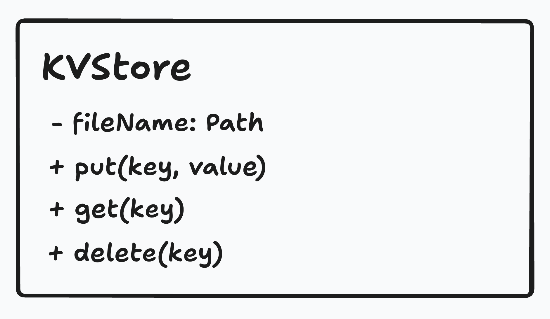
Each time a write is made to the LSMTree, we can append quickly to the end of the file that fileName points to. However, for get() and delete(), we need to traverse the entire file to find the key to delete.

To make this faster, we can use an index. We can store the key along with the line number of the latest modification to the key. For example, if we delete it, we can append a delete line, and when we call get(), we find the deleted row and can tell the user that it doesn’t exist.

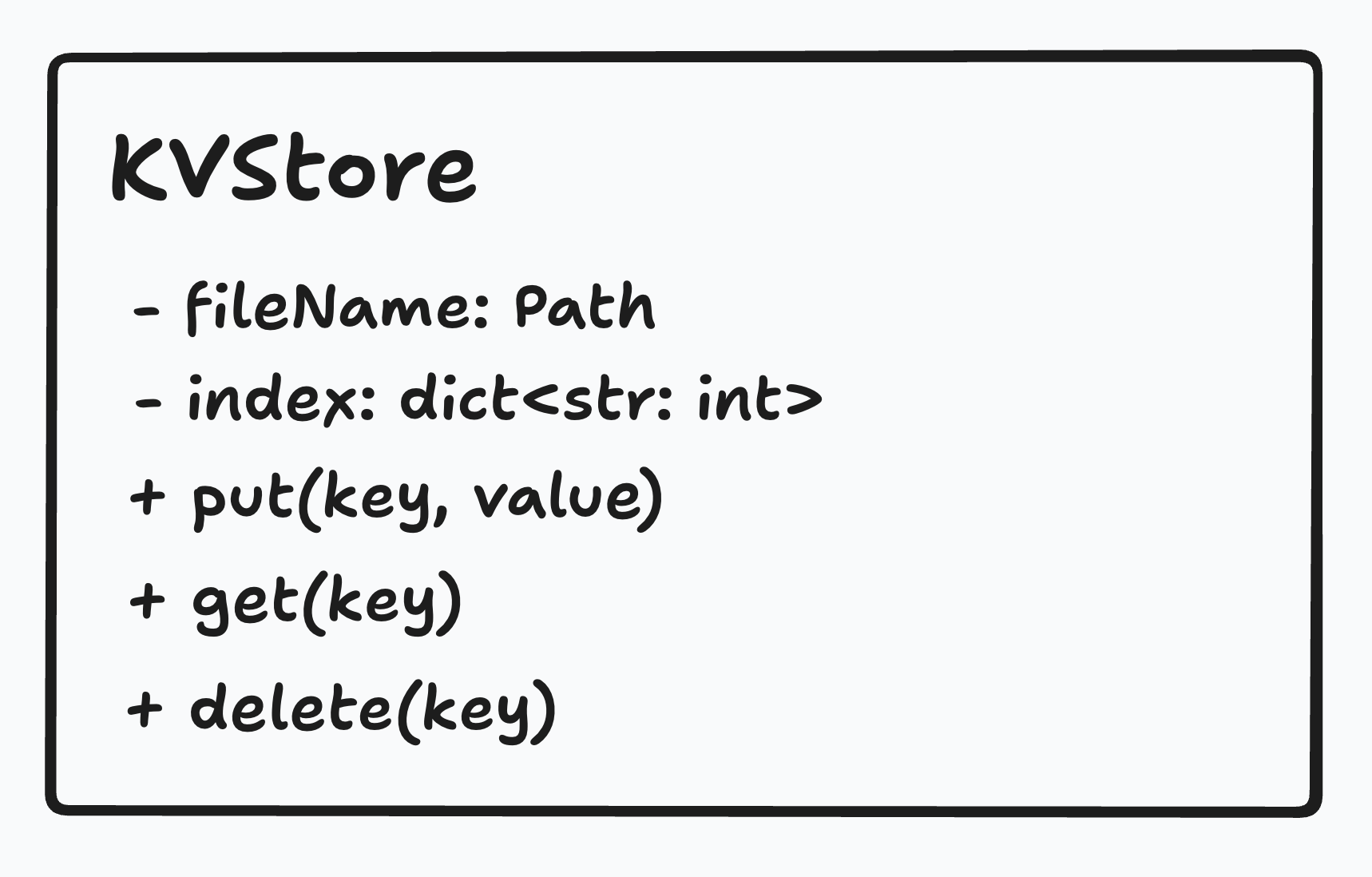
This allows for O(1) time complexity for all operations. At scale, with billions of rows, the index can get quite large and not fit in memory. We need a better way to store our index. One idea is to sort our keys and have sorted blocks of keys point to a file. This lets us reduce the index to the first key of each block that maps to what file it resides in.

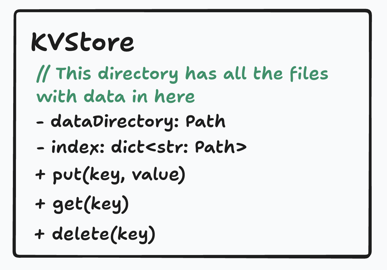
This means that for every key, we insert the key-value pair into the block that it belongs to in a sorted order. This allows for very quick reads at scale but introduces slowness for writes. When many writes are appended to a single file, that file can eventually become too large and require its data to be reorganized across other files. As a result, adding just one key-value pair may trigger multiple writes to storage—an effect known as write amplification.

Up until now, we have been abstracting our storage into files. Files are OS-level abstractions for data but are really composed of fixed blocks on disk. Storage devices read and write one block of data at a time, so from now on, we will refer to our data as blocks on our disk.

Memtable

It would be great if we could preserve fast reads at scale while still supporting writes at a reasonable speed. To do this, we can collect incoming writes in a memtable, an in-memory buffer that keeps key-value pairs sorted. Once the memtable is full, its contents are written to disk as a batch, reducing the number of slow disk operations. Reads then check both the memtable and the indexed data on disk in parallel.

This buffer needs to be implemented in such a way that retrieval and insertion are quick. Skip lists are a good data structure to allow for fast access and insertion of sorted data.

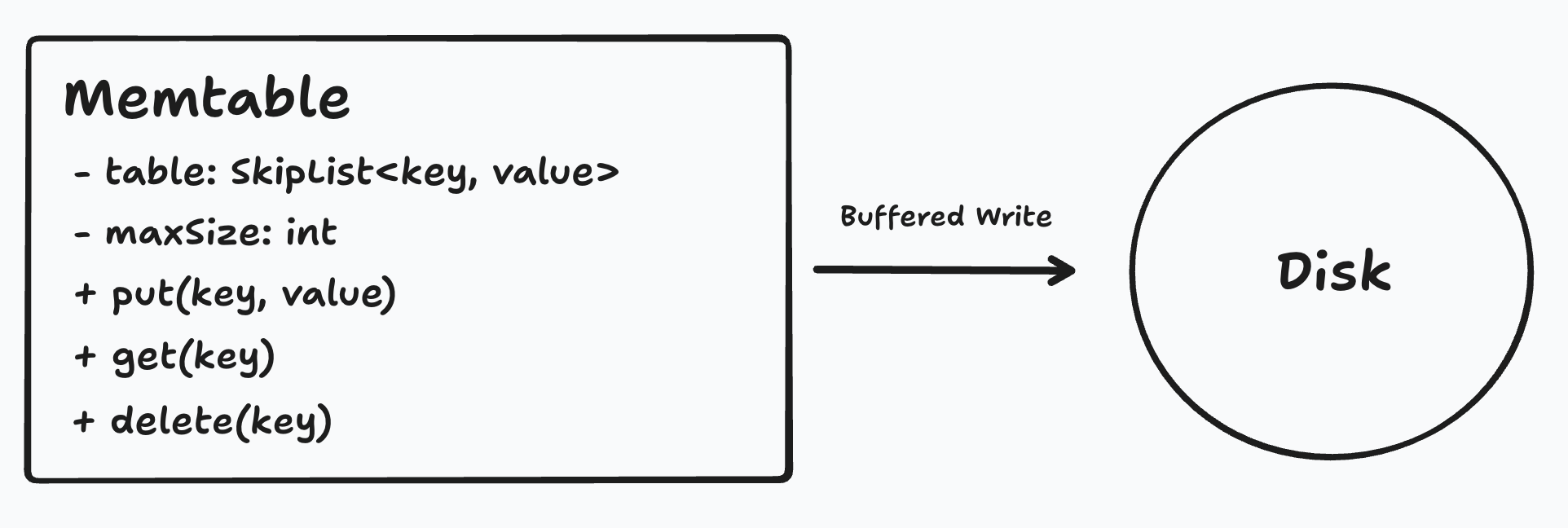
This is a great optimization, but the memtable is stored in memory and is therefore not durable. To make writes recoverable, we first append each update to a log on disk and then apply it to the memtable. If the database crashes, it can replay the log to restore those writes. This is known as the write-ahead log (WAL).

When the active memtable becomes full, it is marked as immutable and a new active memtable begins accepting writes. The immutable memtable is then flushed to disk as an SSTable, allowing writes to continue during the flush.

The flushed file is called a Sorted String Table, or SSTable.

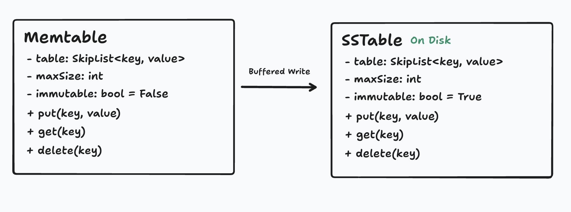
Reads temporarily check both memtables. Immutability makes this manageable: the flushing thread can serialize the old memtable while readers continue using it, knowing that its contents will not change.

Flushing sorted data to disk

The sorted strings in the skip list are split into data blocks that can be written and fetched. We store the sparse index to know which block to pull to get data. The footer stores data on how to read the SSTable.

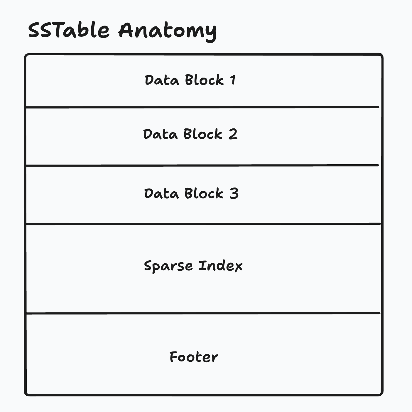
Because the memtable was already sorted, the database can write the SSTable sequentially. We have converted many small, randomly ordered updates into one large sorted write. Writes do not have to stop during the flush. We can flush it and immediately write to the active memtable.

When we have multiple SSTables on disk and we want to read, we will search the SSTables from newest to oldest until we find our key. To delete a key-value pair, we can append a tombstone entry to indicate that it is deleted. Even if multiple copies of the data physically exist in various SSTables, it is logically deleted.

Compaction

Over time, we start to have many copies of a key in different SSTables. This is wasteful, and we can compact SSTables to leave only the most updated version of the key-value pair. We do this by sorting SSTables into a bigger SSTable and getting rid of duplicate entries. This will speed up subsequent scans since there are fewer SSTables to search through. Since SSTables are sorted, we can merge them in linear time.

During compaction, SSTables from one level are merged with overlapping SSTables in the next level. Higher-numbered levels hold more data, and their SSTables generally have non-overlapping key ranges, making reads more efficient.

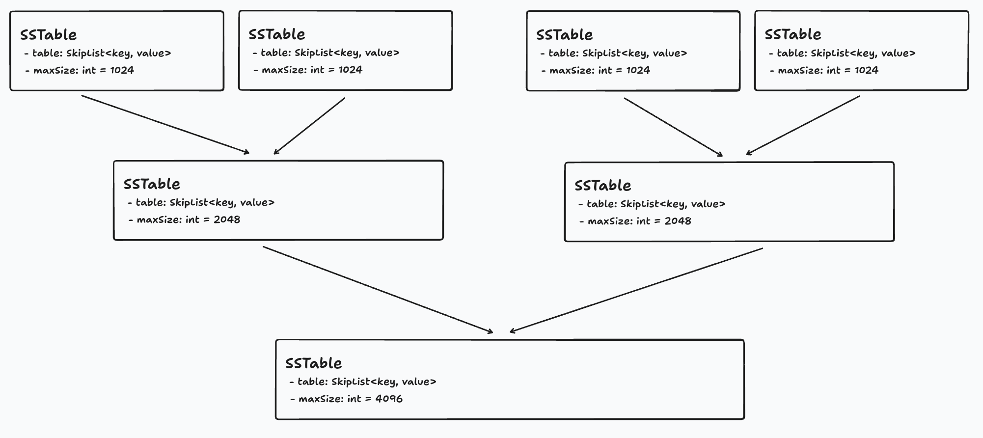
This design works smoothly as long as background flushing and compaction can keep pace with incoming writes. If writes arrive too quickly, Level 0 SSTables accumulate and reads become slower because they must check more files. The database may then throttle or temporarily pause writes to let compaction catch up. This is called a write stall.

Bloom Filters

In our setup, it’s very quick to read data from a theoretical point of view. Reads on an SSTable happen in O(log n). However, in practice, we must do a disk access each time to pull a block of data into memory to operate on. This becomes a bottleneck. We can optimize this using Bloom filters. We can hash all the keys into a long set of bits that act as a fingerprint. Then we can OR them all together to create a fingerprint for a set of keys. This can be done per SSTable. Now, instead of fetching an entire block of data, we can just fetch this SSTable fingerprint, and when we need to get a key, we can check to see that all the bits in the target key’s fingerprint are in the SSTable fingerprint. This will let us quickly rule out SSTables that don’t have the key but may select false positives (which is okay). We can add more bits to the filter to tune the fingerprint to reduce the false-positive rate.

Real Storage Engines

We began with an append-only file because it gave us cheap writes. Each limitation forced the next piece of the design.

1. Scanning was too slow, so we added an index.
2. The index became too large, so we sorted data into blocks.
3. Updating one sorted file was too expensive, so we buffered writes in a memtable.
4. Memory was volatile, so we added a WAL.
5. The memtable was bounded, so we flushed it into immutable SSTables.
6. Multiple files made reads expensive, so we added sparse indexes and Bloom filters.
7. Old versions accumulated, so we introduced compaction and levels.

With this, we’ve derived a very basic LSM Tree—a storage architecture used in many real databases. LevelDB has a simple architecture that mirrors this design. However, we can tune the memtable size, Bloom filters, caches, and other parameters. This is the basis of RocksDB, a more configurable improvement to LevelDB. At a certain scale, we may want to distribute our key-value store onto multiple machines because of the scale of data we have. Cassandra is an implementation similar to RocksDB that supports writes to a set of distributed nodes. It uses Raft consensus to persist writes, and the storage engine logic is much more intertwined with the data propagation. However, these complex systems can run into resource allocation issues. Write stalls become a much bigger problem, which can lead to high tail latency. ScyllaDB introduces sharding of work by CPU core to solve this.

There are many similar databases that rely on the LSM Tree. Understanding where the core architecture excels and falls short can help make tradeoffs in deciding which storage architecture to use.